こちらはこの章のコード例です。これらのページは現在、時間をかけて更新されています(画像、キャプションの追加、おそらくさらなる例の追加)。更新のためにもう一度訪れてください。もちろん、このページを説明が得られる本と一緒に使用するのが最善の方法です。
最近は画像の再アップロードが必要です
単純な変換のテスト
\documentclass[tikz,border=10pt]{standalone}
\usetikzlibrary{calc}
\begin{document}
\begin{tikzpicture}
  \draw[thin,dotted] (-1,-1) grid (3,3);
  \draw[->] (-1,0) -- (3.2,0);
  \draw[->] (0,-1) -- (0,3.2);
  \draw[yshift=2cm] (0,0) -- (1,1);
  \draw[xshift=1cm, yshift=2cm] (0,0) circle(1);
  \draw[shift={(1cm,2cm)}] (0,0) circle(1);
  \draw ([shift={(2,3)}]1,1) -- (4,5);
  \draw ($(1,1)+(3,4)$) -- (4,5);
  \coordinate (A) at (-3, 1);
  \coordinate (B) at (-1, 1);
  \draw (A) -- (B) node[pos=0.5, yshift=2mm] {テキスト};
  \draw[yshift=2cm] (A) -- (B);
  \draw ([yshift=2cm]A.east) -- ([yshift=2cm]B.west);
\end{tikzpicture}
\end{document}
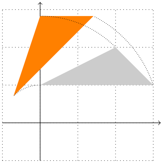
図11.1 – 原点を中心に回転した三角形
\documentclass[tikz,border=10pt]{standalone}
\begin{document}
\begin{tikzpicture}
  % グリッドと座標軸:
  \draw[thin,dotted] (-1,-1) grid (3,3);
  \draw[->] (-1,0) -- (3,0);
  \draw[->] (0,-1) -- (0,3);
  % 元の三角形:
  \fill[gray!40] (0,1) -- (3,1) -- (2,2) --cycle;
  % 回転した三角形:
  \fill[orange, rotate=45] (0,1) -- (3,1) -- (2,2) --cycle;
  % 回転を示すために切り取られた円:
  \begin{scope}
    \clip (0,1) rectangle (3,2.82);
    \draw[densely dotted] circle(3.16);
  \end{scope>
  \begin{scope}
    \clip (0,3) rectangle (2,2);
    \draw[densely dotted] circle(2.83);
  \end{scope>
  \begin{scope}
    \clip (-0.7,0.6) rectangle (0,1);
    \draw[densely dotted] circle(1);
  \end{scope>
\end{tikzpicture}
\end{document}
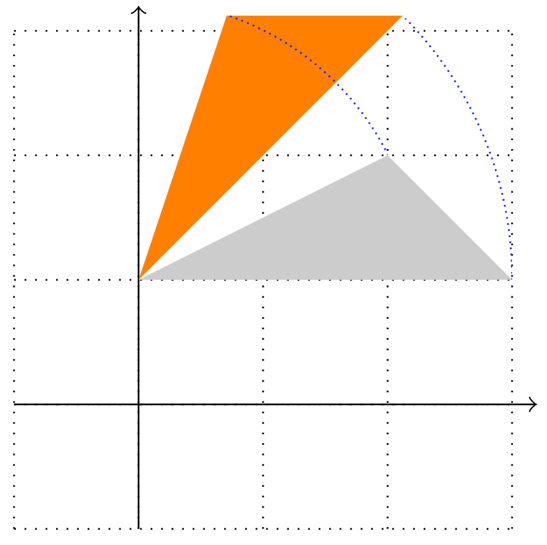
図11.2 – 点を中心に回転した三角形
\documentclass[tikz,border=10pt]{standalone}
\begin{document}
\begin{tikzpicture}
  \draw[thin,dotted] (-1,-1) grid (3,3);
  \draw[->] (-1,0) -- (3.2,0);
  \draw[->] (0,-1) -- (0,3.2);
  % 元の三角形:
  \fill[gray!40] (0,1) -- (3,1) -- (2,2) --cycle;
  % 回転した三角形:
  \fill[orange,rotate around={45:(0,1)}]
    (0,1) -- (3,1) -- (2,2) --cycle;
  % 回転を示すために切り取られた円:
  \begin{scope}
    \clip (2.1,3.1) rectangle (3,1);
    \draw[blue, densely dotted] (0,1) circle(3);
  \end{scope}
  \begin{scope}
    \clip (0.72,3.2) rectangle (2,2);
    \draw[blue, densely dotted] (0,1) circle(2.24);
  \end{scope}
\end{tikzpicture}
\end{document}
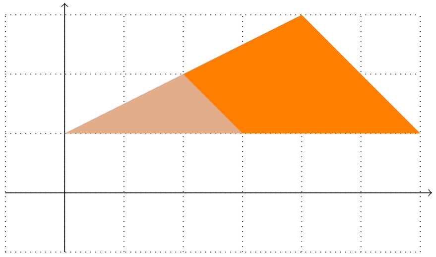
図11.3 – スケーリングされた三角形
\documentclass[tikz,border=10pt]{standalone}
\begin{document}
\begin{tikzpicture}
  \draw[thin,dotted] (-1,-1) grid (6,3);
  \draw[->] (-1,0) -- (6.2,0);
  \draw[->] (0,-1) -- (0,3.2);
  % スケールされた三角形:
  \fill[orange, scale around={2:(0,1)}]
    (0,1) -- (3,1) -- (2,2) --cycle;
  % 元の三角形:
  \fill[gray!40,opacity=0.6] (0,1) -- (3,1) -- (2,2) --cycle;
\end{tikzpicture}
\end{document}

図11.4 – 反転されたスコープ
\documentclass[tikz,border=10pt]{standalone}
\usepackage{tikzducks}
\begin{document}
\begin{tikzpicture}
  \begin{scope}[xscale=-1,transform shape]
    \duck[laughing,speech={\tiny Oh a mirror!}]
  \end{scope}
\end{tikzpicture}
\end{document}
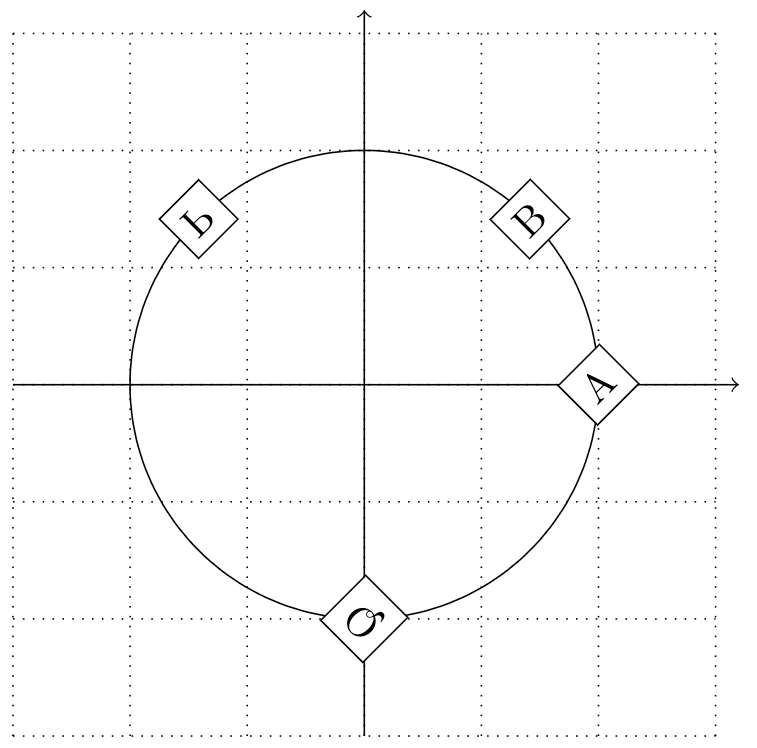
図11.5 – 複数の変形が施されたノード
\documentclass[tikz,border=10pt]{standalone}
\usepackage{tikzducks}
\begin{document}
\begin{tikzpicture}[transform shape, every node/.style={draw, fill=white}]
  \draw[thin,dotted] (-3,-3) grid (3,3);
  \draw[->] (-3,0) -- (3.2,0);
  \draw[->] (0,-3) -- (0,3.2);
  \draw circle(2);
  \node[xshift=2cm, rotate=45] {A};
  \node[rotate=45, xshift=2cm] {B};
  \node[rotate=45, yshift=2cm, yscale=-1] {P};
  \node[yscale=-1, yshift=2cm, rotate=45] {Q};
\end{tikzpicture}
\end{document}
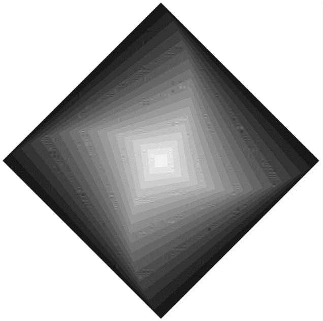
図11.6 – 回転とスケールが適用された正方形
\documentclass[tikz,border=10pt]{standalone}
\usetikzlibrary{positioning}
\begin{document}
\begin{tikzpicture}
  \foreach \i in {90,85,...,5}
    \node[fill=black!\i, scale=\i, rotate=\i/2] {};
\end{tikzpicture}
\end{document}
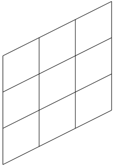
図11.7 – 傾斜された3×3グリッド
\documentclass[tikz,border=10pt]{standalone}
\usetikzlibrary{positioning}
\begin{document}
\begin{tikzpicture}
%  \draw[thin,dotted] (-3,-3) grid (3,3);
%  \draw[->] (-3,0) -- (3,0);
%  \draw[->] (0,-3) -- (0,3);
  \draw[yslant=0.5] (0,0) grid +(3,3);
\end{tikzpicture}
\end{document}
スラントテスト
\documentclass[tikz,border=10pt]{standalone}
\usetikzlibrary{calc}
\begin{document}
\begin{tikzpicture}
  \draw[thin,dotted] (-1,-1) grid (3,3);
  \draw[->] (-1,0) -- (3.2,0);
  \draw[->] (0,-1) -- (0,3.2);
  \filldraw[yslant=1] (0,0) circle (0.3) node [right] {1}
    (1,0) circle (0.3) node [right] {2}
    (1,0) circle (0.3) node [right] {3}
    (3,0) circle (0.3) node [right] {4}
    (0,1) circle (0.3) node [right] {5}
   ;
\end{tikzpicture}
\end{document}
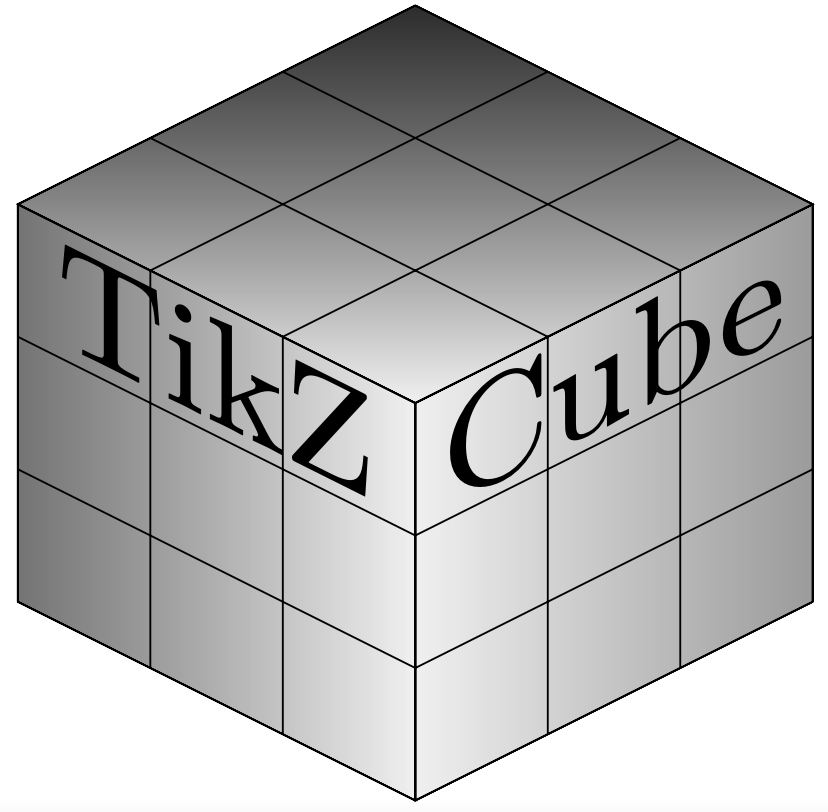
図11.8 – スラントグリッドから作成されたキューブ
\documentclass[tikz,border=10pt]{standalone}
\usetikzlibrary{positioning}
\begin{document}
\begin{tikzpicture}
  \draw[yslant=0.5,
    left color=gray!10, right color=gray!70]
    (3,-3) rectangle +(3,3)
    (3,-3)   grid    +(3,3);
  \draw[yslant=-0.5,
    left color=black!50, right color=gray!10]
    (0,0) rectangle +(3,3)
    (0,0) grid +(3,3);
  \draw[yslant=0.5,xslant=-1,
    bottom color=gray!10, top color=black!80]
    (3,0) rectangle +(3,3)
    (3,0) grid +(3,3);
  \node[yslant=-0.5, scale=3.2]
    at (1.5,1.75) {TikZ};
  \node[yslant= 0.5, scale=3.2]
    at (4.5,1.75) {キューブ};
\end{tikzpicture}
\end{document}
変化なしの変形
\documentclass[border=10pt]{standalone}
\usepackage{tikz}
\usetikzlibrary{positioning}
\begin{document}
\begin{tikzpicture}
  \node (tex) [fill=orange, text=white] {TEX};
  \node (pdf) [fill={rgb:red,244;green,15;blue,2},
    text=white, right=of tex] {PDF};
  \draw (tex) edge[->,yshift= 0.1mm, rotate= 4] (pdf);
  \draw (tex) edge[->,yshift=-0.1mm, rotate=-4] (pdf);
\end{tikzpicture}
\end{document}

図11.9 – 変形された矢印
\documentclass[border=10pt]{standalone}
\usepackage{tikz}
\usetikzlibrary{positioning}
\begin{document}
\begin{tikzpicture}
  \node (tex) [fill=orange, text=white] {TEX};
  \node (pdf) [fill={rgb:red,244;green,15;blue,2},
    text=white, right=of tex] {PDF};
  \draw (tex) edge[->,transform canvas={yshift= 0.1mm,rotate=4}] (pdf);
  \draw (tex) edge[->,transform canvas={yshift=-0.1mm,rotate=-4}] (pdf);
\end{tikzpicture}
\end{document}
次の章 へ進む.