こちらはこの章のコード例です。これらのページは現在、時間をかけて更新されています(画像、キャプションの追加、おそらくさらなる例の追加)。更新のためにもう一度訪れてください。もちろん、このページを説明が得られる本と一緒に使用するのが最善の方法です。
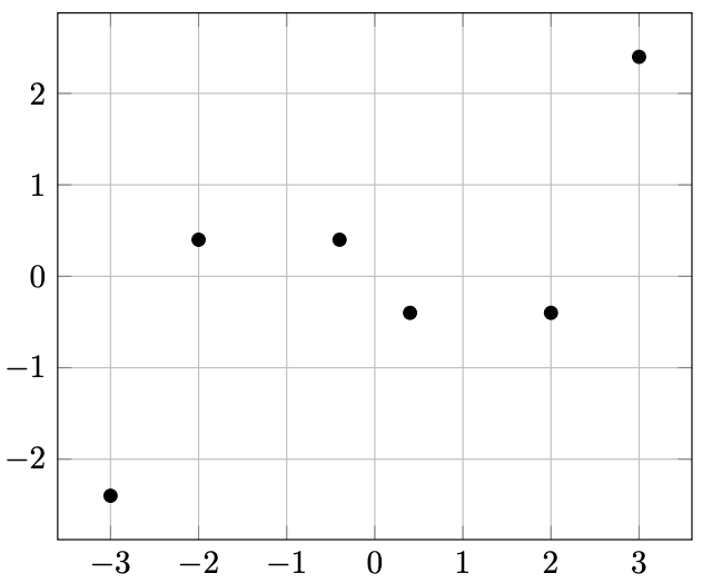
図 13.1 – 座標のプロット
\documentclass[tikz,border=10pt]{standalone}
\usepackage{pgfplots}
\pgfplotsset{compat=1.18}
\begin{document}
\begin{tikzpicture}
  \begin{axis}[grid]
    \addplot[only marks] coordinates
      { (-3,-2.4)  (-2,0.4) (-0.4,0.4)
        (0.4,-0.4) (2,-0.4) (3,2.4) };
  \end{axis}
\end{tikzpicture}
\end{document}
クラシックなTikZでのプロット
\documentclass[tikz,border=10pt]{standalone}
\begin{document}
\begin{tikzpicture}
  \draw[->] (-3,0) -- (3,0);
  \draw[->] (0,-3) -- (0,3);
  \foreach \i in {-3,-2,-1,1,2,3} {
    \node at (\i,-0.2) {\i};
    \node at (-0.2,\i) {\i};
  }
  \draw[domain=-3:3, samples=50, thick] plot (\x, \x^3/5 - \x);
\end{tikzpicture}
\end{document}
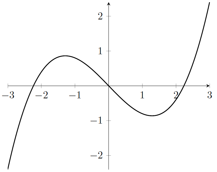
図 13.2 – 中心にx軸とy軸がある立方プロット
\documentclass[tikz,border=10pt]{standalone}
\usepackage{pgfplots}
\begin{document}
\begin{tikzpicture}
  \begin{axis}[axis lines=center]
    \addplot[samples=80, smooth, thick, domain=-3:3]
      {x^3/5 - x};
  \end{axis}
\end{tikzpicture}
\end{document}
プロットスタイルの定義
\documentclass[tikz,border=10pt]{standalone}
\usepackage{pgfplots}
\pgfplotsset{every axis plot post/.append style =
  {samples=80, smooth, thick, black, mark=none} }
\begin{document}
\begin{tikzpicture}
  \begin{axis}[axis lines = center, domain = -3:3]
    \addplot {x^3/5 - x};
  \end{axis}
\end{tikzpicture}
\end{document}
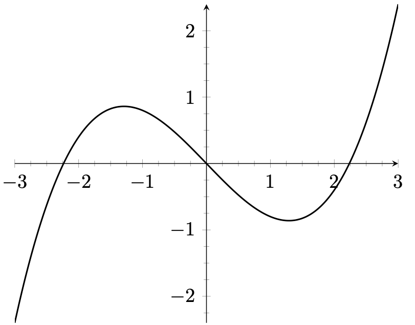
図 13.3 – 小さい目盛り付きの軸
\documentclass[tikz,border=10pt]{standalone}
\usepackage{pgfplots}
\begin{document}
\begin{tikzpicture}
  \begin{axis}[axis lines=center, minor tick num=3]
    \addplot[samples=80, smooth, thick, domain=-3:3]
      {x^3/5 - x};
  \end{axis}
\end{tikzpicture}
\end{document}
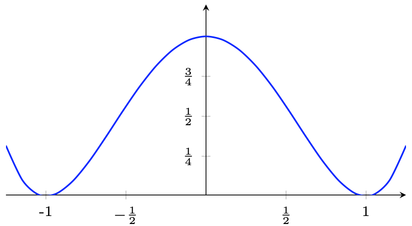
図 13.4 – カスタマイズされた目盛り
\documentclass[tikz,border=10pt]{standalone}
\usepackage{pgfplots}
\pgfplotsset{every axis plot post/.append style={thick,smooth,mark=none}}
\begin{document}
\begin{tikzpicture}
  \begin{axis}[axis lines = middle, axis equal image,
    domain = -1.25:1.25, y domain = 0:1.25,
    ymax = 1.2,
    tick label style = {font=\scriptsize},
    xtick = {-1, -0.5, 0.5, 1},
    xticklabels = {-1, $-\frac{1}{2}$, $\frac{1}{2}$, 1},
    ytick = {0.25, 0.5, 0.75},
    yticklabels = {$\frac{1}{4}$, $\frac{1}{2}$,
    $\frac{3}{4}$} ]
  \addplot { (x^2-1)^2 };
\end{axis}
\end{tikzpicture}
\end{document}
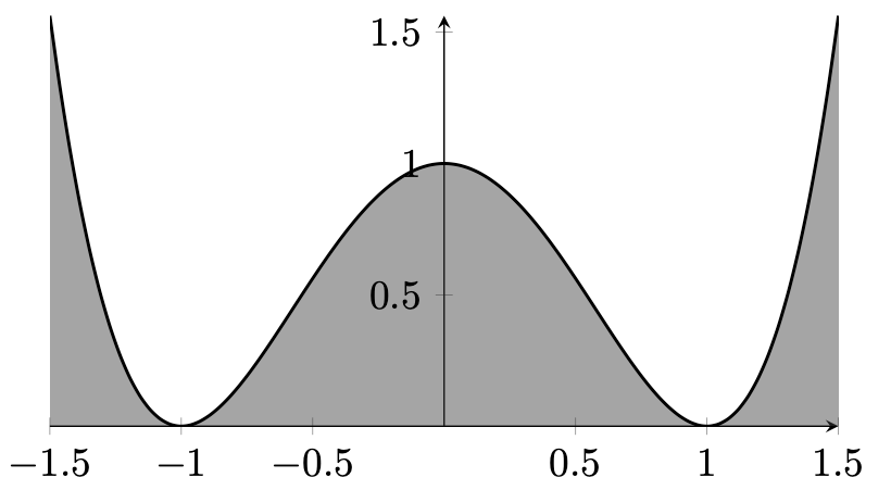
図 13.5 – プロットの下の領域の塗りつぶし
\documentclass[tikz,border=10pt]{standalone}
\usepackage{pgfplots}
\usepgfplotslibrary{fillbetween}
\pgfplotsset{every axis plot post/.append style =
  {samples=80, smooth, thick, black, mark=none} }
\begin{document}
\begin{tikzpicture}
\begin{axis}[axis lines = center,
  axis equal image, domain = -1.5:1.5]
  \addplot[name path=quartic] {(x^2-1)^2};
  \path[name path=xaxis] (axis cs:-1.6,0)
    -- (axis cs:1.6,0);
  \addplot[darkgray, opacity=0.5]
    fill between[of=quartic and xaxis];
\end{axis}
\end{tikzpicture}
\end{document}
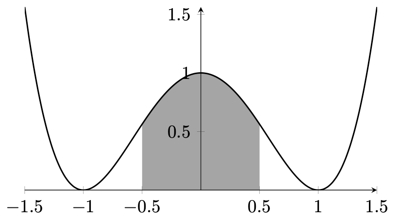
図 13.6 – プロット下のセグメントの塗りつぶし
\documentclass[tikz,border=10pt]{standalone}
\usepackage{pgfplots}
\usepgfplotslibrary{fillbetween}
\pgfplotsset{every axis plot post/.append style =
  {samples=80, smooth, thick, black, mark=none} }
\begin{document}
\begin{tikzpicture}
\begin{axis}[axis lines = center,
  axis equal image, domain = -1.5:1.5]
  \addplot[name path=quartic] {(x^2-1)^2};
  \path[name path=xaxis] (axis cs:-1.6,0)
    -- (axis cs:1.6,0);
  \addplot[darkgray, opacity=0.5]
    fill between[of=quartic and xaxis,
    soft clip = {domain=-0.5:0.5} ];
\end{axis}
\end{tikzpicture}
\end{document}
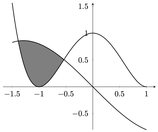
図 13.7 – プロット間の領域の塗りつぶし
\documentclass[tikz,border=10pt]{standalone}
\usepackage{pgfplots}
\usepgfplotslibrary{fillbetween}
\pgfplotsset{every axis plot post/.append style =
  {samples=80, smooth, thick, black, mark=none} }
\begin{document}
\begin{tikzpicture}
  \begin{axis}[axis lines = center, axis equal,
      domain = -1.5:1]
    \addplot[name path=cubic]   {x^3/5 - x};
    \addplot[name path=quartic] {(x^2-1)^2};
    \addplot fill between[of=cubic and quartic, split,
      every segment/.style      = {transparent},
      every segment no 1/.style = {gray, opaque}];
  \end{axis}
\end{tikzpicture}
\end{document}
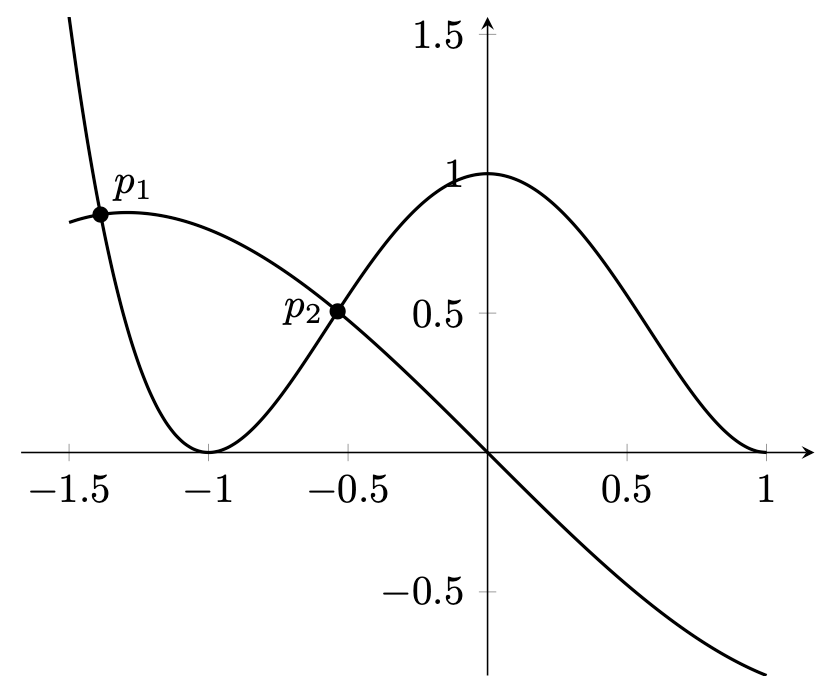
図 13.8 – プロットの交点
\documentclass[border=10pt]{standalone}
\usepackage{pgfplots}
\usetikzlibrary{intersections}
\pgfplotsset{every axis plot post/.append style =
  {samples=80, smooth, thick, black, mark=none} }
\begin{document}
\begin{tikzpicture}
  \begin{axis}[axis lines = center, axis equal,
      domain = -1.5:1]
    \addplot[name path=cubic]   {x^3/5 - x};
    \addplot[name path=quartic] {(x^2-1)^2};
    \fill[name intersections = {of=cubic and quartic,
     name=p}]
      (p-1) circle (2pt) node [above right] {$p_1$}
      (p-2) circle (2pt) node [left]        {$p_2$};
\end{axis}
\end{tikzpicture}
\end{document}
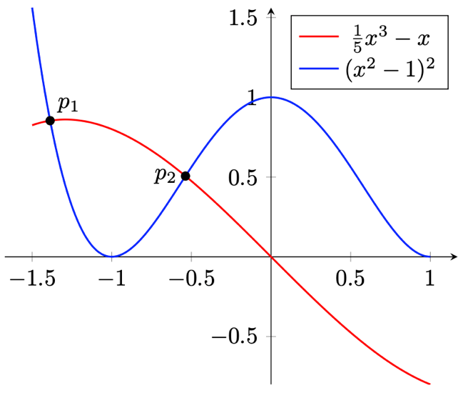
図 13.9 – 凡例付きのプロット
\documentclass[border=10pt]{standalone}
\usepackage{pgfplots}
\usetikzlibrary{intersections}
\pgfplotsset{every axis plot post/.append style =
  {samples=80, smooth, thick, mark=none} }
\begin{document}
\begin{tikzpicture}
  \begin{axis}[axis lines = center, axis equal,
      domain = -1.5:1,
      legend entries = {$\frac{1}{5}x^3-x$, $(x^2-1)^2$}]
    \addplot[red,  name path=cubic] {x^3/5 - x};
    \addplot[blue, name path=quartic] {(x^2-1)^2};
    \fill[name intersections = {of=cubic and quartic,
     name=p}]
      (p-1) circle (2pt) node [above right] {$p_1$}
      (p-2) circle (2pt) node [left]        {$p_2$};
  \end{axis}
\end{tikzpicture}
\end{document}
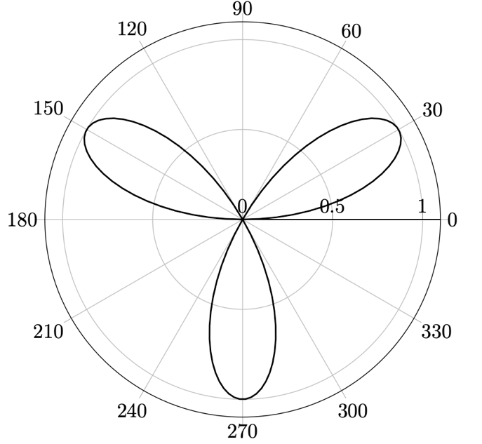
図 13.10 – 極座標系における三角関数のプロット
\documentclass[border=10pt]{standalone}
\usepackage{pgfplots}
\usepgfplotslibrary{polar}
\begin{document}
\begin{tikzpicture}
\begin{polaraxis}
  \addplot[domain=0:180, samples=100, thick] {sin(3*x)};
\end{polaraxis}
\end{tikzpicture}
\end{document}
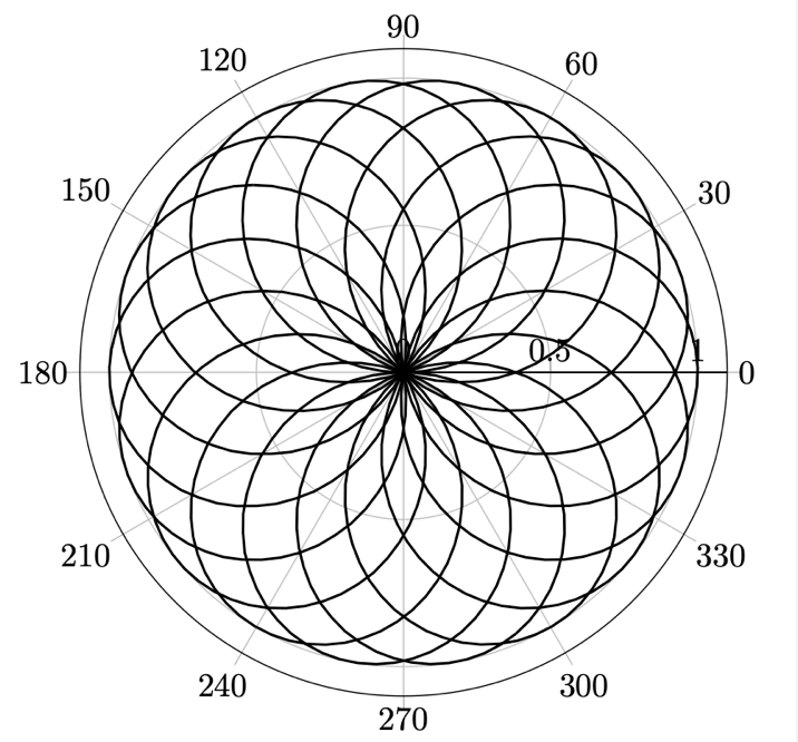
図 13.11 – 複数回の360度を超える三角関数
\documentclass[border=10pt]{standalone}
\usepackage{pgfplots}
\usepgfplotslibrary{polar}
\begin{document}
\begin{tikzpicture}
\begin{polaraxis}
  \addplot[domain=0:2880, samples=800, thick] {sin(9*x/8)};
\end{polaraxis}
\end{tikzpicture}
\end{document}
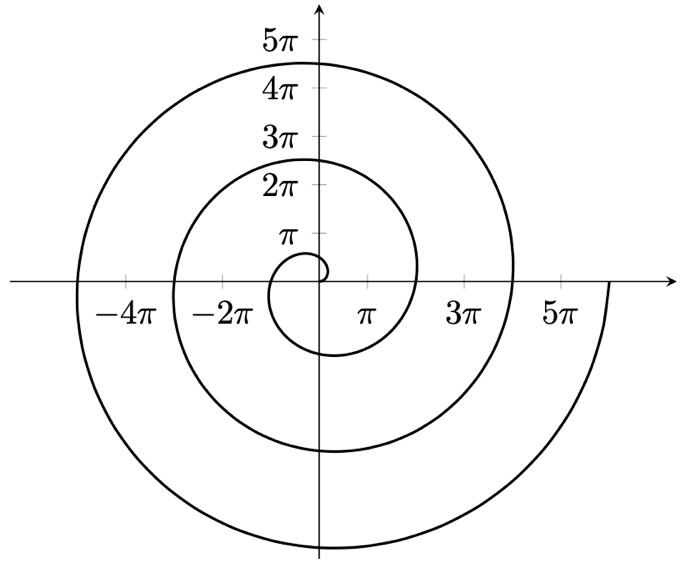
図 13.12 – アルキメデスの螺旋
\documentclass[border=10pt]{standalone}
\usepackage{pgfplots}
\pgfplotsset{trig format plots=rad}
\begin{document}
\begin{tikzpicture}
  \begin{axis}[axis lines = middle, axis equal,
      domain = 0:6*pi, ymin=-18, ymax=18,
      xtick = {-4*pi,-2*pi,pi,3*pi,5*pi},
      ytick = {pi, 2*pi, 3*pi, 4*pi, 5*pi},
      xticklabels = {$-4\pi$, $-2\pi$,
        $\vphantom{1}\pi$, $3\pi$, $5\pi$},
      yticklabels = {$\vphantom{1}\pi$, $2\pi$,
        $3\pi$, $4\pi$, $5\pi$}
    ]
    \addplot[samples=120, smooth, thick, variable=t]
      ( {t*cos(t)}, {t*sin(t)} );
\end{axis}
\end{tikzpicture}
\end{document}
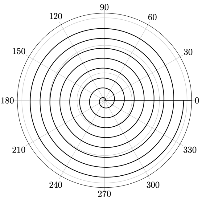
図 13.13 – 極座標系におけるアルキメデスの螺旋
\documentclass[border=10pt]{standalone}
\usepackage{pgfplots}
\pgfplotsset{compat=1.18}
\usepgfplotslibrary{polar}
\begin{document}
\begin{tikzpicture}
  \begin{polaraxis}[yticklabel=\empty]
    \addplot[domain=0:2880, samples=200, smooth, thick] {x};
  \end{polaraxis}
\end{tikzpicture}
\end{document}
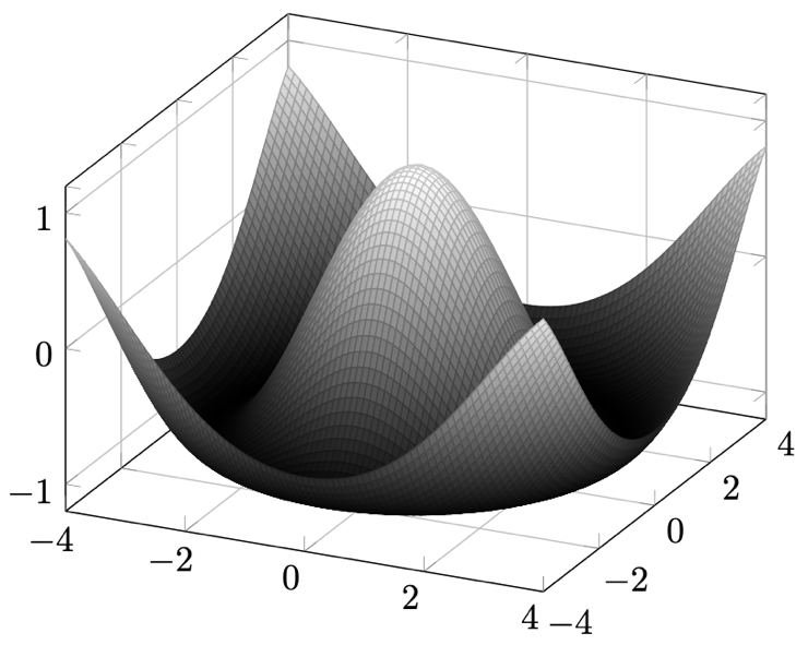
図 13.14 – 3D座標系におけるプロット
\documentclass[border=10pt]{standalone}
\usepackage{pgfplots}
\usepgfplotslibrary{colormaps}
\pgfplotsset{trig format plots=rad}
\begin{document}
\begin{tikzpicture}
  \begin{axis}[
      domain    = -4:4, samples    = 70,
      y domain  = -4:4, samples y  = 70,
      colormap/blackwhite, grid]
    \addplot3[surf] { cos(sqrt(x^2+y^2)) };
  \end{axis}
\end{tikzpicture}
\end{document}
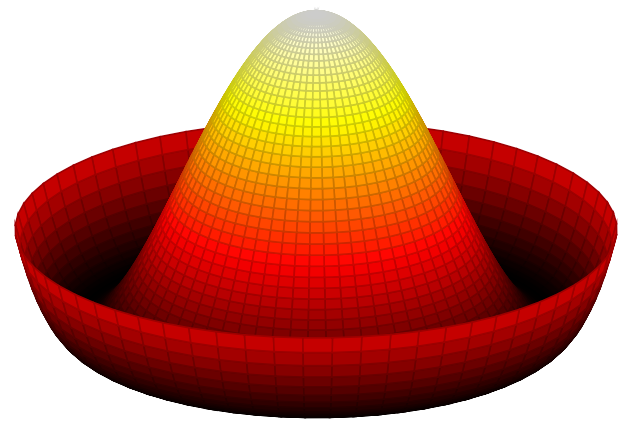
図 13.15 – ソンブレロプロット
\documentclass[tikz,border=10pt]{standalone}
\usepackage:pgfplots}
\usepgfplotslibrary{colormaps}
\begin{document}
  \begin{tikzpicture}
    \begin{axis}[hide axis, colormap/hot2]
      \addplot3 [surf, z buffer=sort, trig format plots=rad,
        samples=65, domain=-pi:pi, y domain=0:1.25,
        variable=t, variable y=r]
        ({r*sin(t)}, {r*cos(t)}, {(r^2-1)^2});
    \end{axis}
  \end{tikzpicture}
\end{document}
次の章 へ進む.
これはgnuplotを使用してプロットする方法が記載されています:Mexican hat potential polar.svg は 自発的対称性の破れ(ソンブレロポテンシャル)に関するWikipediaの記事からです。