ノードの位置決めと描画

こちらはこの章のコード例です。これらのページは現在、時間をかけて更新されています（画像、キャプションの追加、おそらくさらなる例の追加）。更新のためにもう一度訪れてください。もちろん、このページを説明が得られる本と一緒に使用するのが最善の方法です。

---

図 3.1 – 色付きのノード

\documentclass[tikz,border=10pt]{standalone}
\begin{document}
\begin{tikzpicture}
  \draw (4,2) node[draw, color=red, fill=yellow, text=blue] {TikZ};
\end{tikzpicture}
\end{document}

---

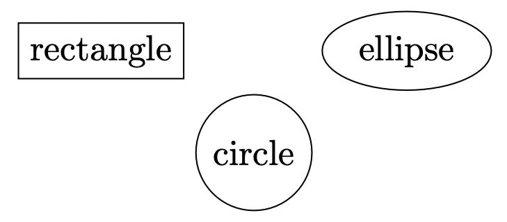
図 3.2 – 異なる形のノード

\documentclass[tikz,border=10pt]{standalone}
\usetikzlibrary{shapes}
\begin{document}
\begin{tikzpicture}
  \node (r) at (0,1)   [draw, rectangle] {rectangle};
  \node (c) at (1.5,0) [draw, circle]    {circle};
  \node (e) at (3,1)   [draw, ellipse]   {ellipse};
\end{tikzpicture}
\end{document}

---

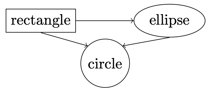
図 3.3 – 矢印付きのノード

\documentclass[tikz,border=10pt]{standalone}
\usetikzlibrary{shapes}
\begin{document}
\begin{tikzpicture}
  \node (r) at (0,1)   [draw, rectangle] {rectangle};
  \node (c) at (1.5,0) [draw, circle]    {circle};
  \node (e) at (3,1)   [draw, ellipse]   {ellipse};
  \draw[->] (r.east)  -- (e.west);
  \draw[->] (r.south) -- (c.north west);
  \draw[->] (e.south) -- (c.north east);
\end{tikzpicture}
\end{document}

---

図 3.4 – デフォルトのアンカー

\documentclass[tikz,border=10pt]{standalone}
\begin{document}
\begin{tikzpicture}
\draw[fill=red] (4,2) circle[radius=0.1];
\node at (4,2) [draw, rectangle] {rectangle};
\end{tikzpicture}
\end{document}

---

図 3.5 – 南西アンカー

\documentclass[tikz,border=10pt]{standalone}
\begin{document}
\begin{tikzpicture}
  \draw[fill=red] (4,2) circle[radius=0.1];
  \node at (4,2) [draw, rectangle, anchor=south west]
    {rectangle};
\end{tikzpicture}
\end{document}

---

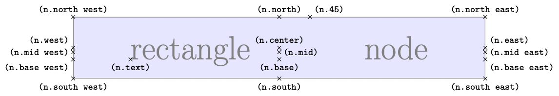
図 3.6 – アンカー付きの四角形

\documentclass[tikz,border=5]{standalone}
\usetikzlibrary{positioning}
\tikzset{shape example/.style = {
    color=black!50, draw, fill=blue!10,
    inner xsep=1.5cm, inner ysep=0.5cm,
}}
\begin{document}
\Huge
\begin{tikzpicture}[node distance = 1mm]
  \node[name=n,shape=rectangle,shape example]
    {\Huge rectan\smash{g}le\hspace{3cm}node};
  \foreach \anchor/\placement in
    {center/above, text/below, 45/above right,
       mid/right, mid east/right, mid west/left,
       base/below, base east/below right, base west/below left,
       north/above, south/below, east/above right, west/above left,
       north east/above, south east/below, south west/below, north west/above}
      \draw[shift=(n.\anchor)] plot[mark=x] coordinates{(0,0)}
        node[\placement,label distance = 0mm,inner sep=3pt]
          {\scriptsize\texttt{(n.\anchor)}};
\end{tikzpicture}
\end{document}

---

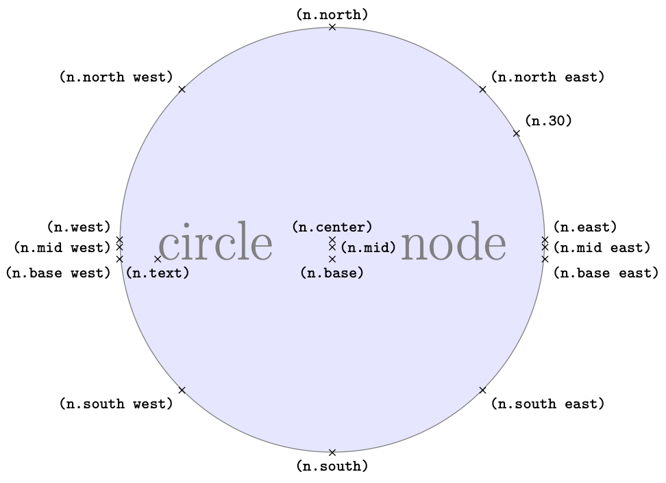
図 3.7 – アンカー付きの円形

\documentclass[tikz,border=5]{standalone}
\usetikzlibrary{positioning}
\tikzset{shape example/.style = {
    color=black!50, draw, fill=blue!10,
    inner xsep=0.5cm, inner ysep=0.5cm,
}}
\begin{document}
\Huge
\begin{tikzpicture}[node distance = 1mm]
  \node[name=n,shape=circle,shape example] {\Huge circle\hspace{2cm}node};
  \foreach \anchor/\placement in
    {center/above, text/below, 30/above right,
       mid/right, mid east/right, mid west/left,
       base/below, base east/below right, base west/below left,
       north/above, south/below, east/above right, west/above left,
       north east/above right, south east/below right, south west/below left,
         north west/above left}
      \draw[shift=(n.\anchor)] plot[mark=x] coordinates{(0,0)}
        node[\placement,label distance = 0mm,inner sep=3pt]
          {\scriptsize\texttt{(n.\anchor)}};
\end{tikzpicture}
\end{document}

---

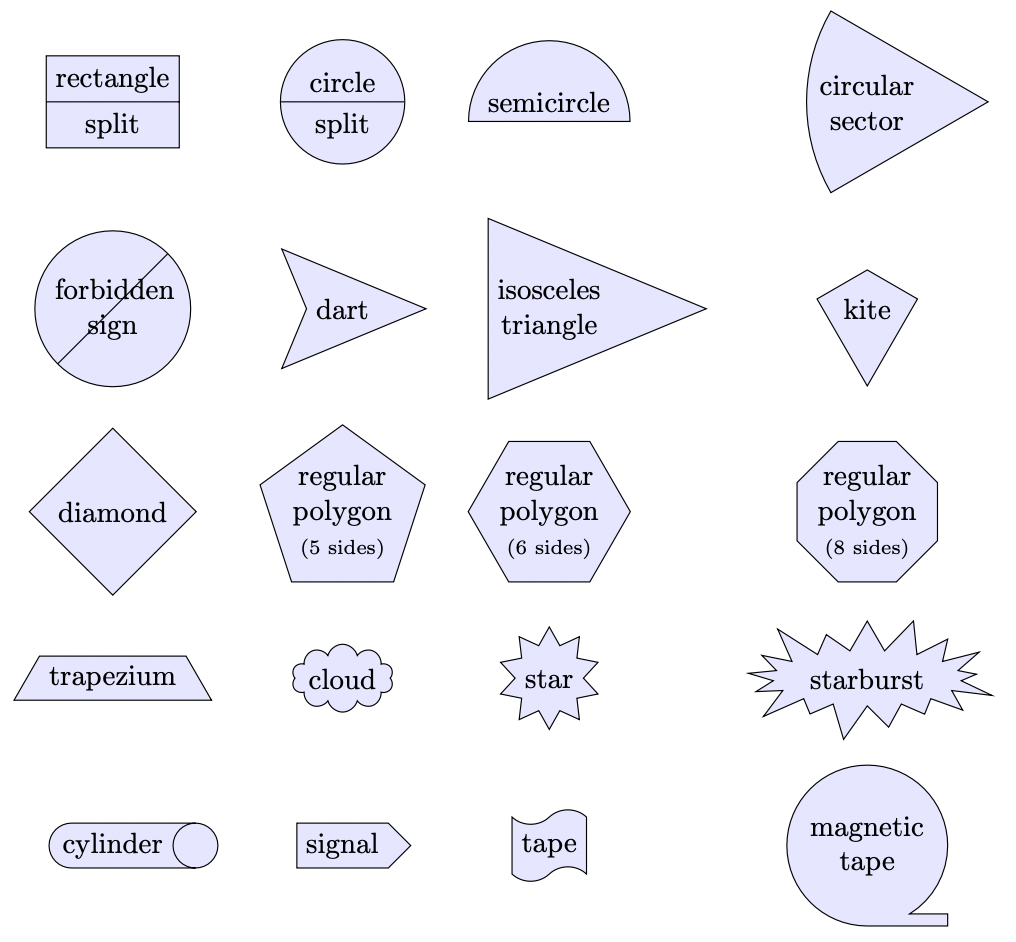
図 3.8 – 様々なノード形状

\documentclass[tikz,border=1pt]{standalone}
\usepackage{tikz}
\usetikzlibrary{shapes,snakes}
\begin{document}
\begin{tikzpicture}
    \matrix[nodes={draw, fill=blue!15},
        row sep=0.2cm, column sep=0.3cm,
        nodes={font=\sffamily}] {
    \node[rectangle split, rectangle split parts=2] {rectangle \nodepart{two} split};&
    \node[circle split] {circle \nodepart{lower} split}; &
    \node[semicircle] {semicircle};&
    \node[circular sector, align=center] {circular\\sector};&
    \\
    \node[forbidden sign,text width=4em, text centered]
                    {forbidden sign};&
    \node[dart] {dart};&
    \node[kite] {kite};&
    \node[isosceles triangle, align=center] {isosceles\\triangle};&
                    \\
    \node[diamond] {diamond};&
    \node[regular polygon, regular polygon sides=5, align=center]
      {regular\\polygon\\(5 sides)};&
    \node[regular polygon, regular polygon sides=6, align=center]
      {regular\\polygon\\(6 sides)};&
    \node[regular polygon, regular polygon sides=8, align=center]
      {regular\\polygon\\(8 sides)};\\
    \node[trapezium] {trapezium};&
    \node[cloud] {cloud};&
    \node[star] {star};&
    \node[starburst] {starburst};&
    \\
    \node[cylinder] {cylinder};&
    \node[signal] {signal};&
    \node[tape] {tape};&
    \node[magnetic tape, align=center] {magnetic\\tape};&
    \\
    };
\end{tikzpicture}
\end{document}

---

図 3.9 – ノード形状の配置

\documentclass[tikz,border=10pt]{standalone}
\usepackage{tikzpeople}
\usetikzlibrary{shapes}
\begin{document}
\begin{tikzpicture}
  \node (student) [graduate, monitor, minimum size=2cm] {};
  \node at (student.45) [starburst, draw=red, fill=yellow,
    starburst point height=0.4cm, line width=1pt,
    font=\ttfamily\scriptsize, inner sep=1.5pt] {error};
  \node at (student.130) [cloud callout, cloud puffs=13, aspect=3,
    anchor=pointer, shading=ball, ball color=darkgray,
    text=white, font=\bfseries] {My thesis...!};
\end{tikzpicture}
\end{document}

---

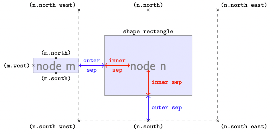
図 3.10 – ノード内外のスペーシング

\documentclass[tikz,border=10pt]{standalone}
\usetikzlibrary{calc}
\begin{document}
\begin{tikzpicture}[font={\scriptsize\ttfamily}]
  \node[draw,rectangle,outer sep=1cm,inner sep=1cm,color=black!50, draw, fill=blue!10]
  (n) {{\sffamily\Large node n}};
  \draw[<->,thick,blue] (n.south)
      --++(0,1cm) node[midway,right]{outer sep};
  \draw[<->,thick,red] (n.south) ++(0,1cm) 
      --++(0,1cm)node[midway,right]{inner sep};
  \node[,outer sep=0,draw,left,color=black!50, draw, fill=blue!10,] 
      (m) at(n.west) {{\sffamily\Large node m}};
  \draw[<->,blue,thick] (m.east) -- ++(1cm,0) node[midway,above] {outer}
    node[midway,below] {sep};
  \draw[<->,red,thick] ($(n.west)+(1,0)$) -- ++(1cm,0) node[midway,above] {inner}
    node[midway,below] {sep};
  \foreach \anchor/\placement in
    {south west/below left,south/below,north/above,north west/above left,
       north east/above right,south east/below right}
       \draw[shift=(n.\anchor)] plot[mark=x] coordinates{(0,0)}
        node[\placement,label distance = 0mm,inner sep=3pt] {(n.\anchor)};
  \foreach \anchor/\placement in
    {west/left,south/below,north/above}
       \draw[shift=(m.\anchor)] plot[mark=x] coordinates{(0,0)}
        node[\placement,label distance = 0mm,inner sep=3pt] {(m.\anchor)};
  \draw[dashed] (n.south west) rectangle (n.north east);
  \node[above] at ($(n.center)!0.5!(n.north)$) {shape rectangle};
\end{tikzpicture}
\end{document}

---

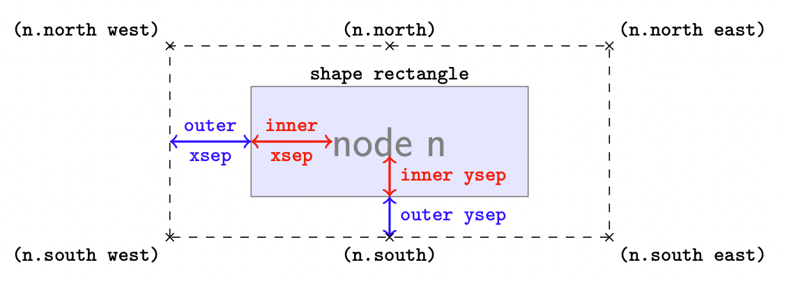
図 3.11 – 異なる水平および垂直スペーシング

\documentclass[tikz,border=10pt]{standalone}
\usetikzlibrary{calc}
\begin{document}
\begin{tikzpicture}[font={\scriptsize\ttfamily}]
  \node[draw,rectangle,outer xsep=1cm,outer ysep=0.5cm,inner xsep=1cm,
    inner ysep=0.5cm,color=black!50, draw, fill=blue!10,] (n) {{\sffamily\Large node n}};
  \draw[<->,thick,blue] (n.south)
      --++(0,0.5cm) node[midway,right]{outer ysep};
  \draw[<->,thick,red] (n.south) ++(0,0.5cm) 
      --++(0,0.5cm)node[midway,right]{inner ysep};    
  \draw[<->,blue,thick] (n.west) -- ++(1cm,0) node[midway,above] {outer}
    node[midway,below] {xsep};
  \draw[<->,red,thick] ($(n.west)+(1,0)$) -- ++(1cm,0) node[midway,above] {inner}
    node[midway,below] {xsep};
  \foreach \anchor/\placement in
    {south west/below left,south/below,north/above,north west/above left,
       north east/above right,south east/below right}
       \draw[shift=(n.\anchor)] plot[mark=x] coordinates{(0,0)}
        node[\placement,label distance = 0mm,inner sep=3pt] {(n.\anchor)};
  \draw[dashed] (n.south west) rectangle (n.north east);
  \node[above] at ($(n.center)!0.5!(n.north)$) {shape rectangle};
\end{tikzpicture}
\end{document}

---

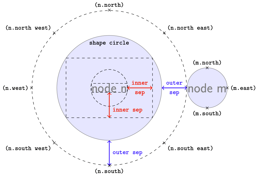
図 3.12 – 円形ノード内外のスペーシング

\documentclass[tikz,border=10pt]{standalone}
\usetikzlibrary{calc}
\newcommand{\n}{\sffamily\Large node n}
\newcommand{\invis}{\phantom{\sffamily\Large node n}}
\begin{document}
\begin{tikzpicture}[font={\scriptsize\ttfamily}]
  % node n
  \node[draw,circle,outer sep=1cm,inner sep=1cm,color=black!50, draw, fill=blue!10] (n) {{\n}};
  % label "shape circle"
  \node[above] at ($(n.center)!0.5!(n.north)$) {shape circle};

  % dashed helper nodes with same position and (invisible) same text
  \node[circle,draw,densely dashed,inner sep=0pt,outer sep=0pt] at (n.center) {\invis};
  \node[rectangle,draw,densely dashed,inner sep=0pt,outer sep=0pt] at (n.center) {\invis};
  \node (o) [rectangle,draw, dashed,inner sep=1cm,outer sep=0pt] at (n.center) {\invis};

  % neighbor node
  \node[circle,inner sep=0,outer sep=0,draw,right,color=black!50, draw, fill=blue!10] 
      (m) at(n.east) {{\sffamily\Large node m}};

  % vertical sep
  \draw[<->,thick,blue] (n.south)
    --++(0,1cm) node[midway,right]{outer sep};
  \draw[<->,thick,red] (o.south)
    -- ++(0,1cm) node[pos=0.3,right]{inner sep};

  % horizontal sep
  \draw[<->,red,thick] (o.east) -- ++(-1cm,0)
    node[midway,above] {inner} node[midway,below] {sep};
  \draw[<->,blue,thick] (m.west) -- ++(-1cm,0)
    node[midway,above] {outer} node[midway,below] {sep};

% some anchors
  \foreach \anchor/\placement in
    {south west/below left,south/below,north/above,north west/above left,
       north east/above right,south east/below right,west/left}
       \draw[shift=(n.\anchor)] plot[mark=x] coordinates{(0,0)}
        node[\placement,label distance = 0mm,inner sep=3pt] {(n.\anchor)};
  \foreach \anchor/\placement in
    {east/right,south/below,north/above}
       \draw[shift=(m.\anchor)] plot[mark=x] coordinates{(0,0)}
        node[\placement,label distance = 0mm,inner sep=3pt] {(m.\anchor)};

% random circle :-)
\draw[dashed] (n.center) circle (3.05cm);
\end{tikzpicture}
\end{document}

---

図 3.13 – 円上のノード

\documentclass[tikz,border=10pt]{standalone}
\begin{document}
\begin{tikzpicture}
  \draw circle [fill, radius=2pt] node [anchor=south] {text};
\end{tikzpicture}
\end{document}

異なるコード、同じ出力:

\documentclass[tikz,border=10pt]{standalone}
\begin{document}
\begin{tikzpicture}
  \draw circle [fill, radius=2pt] node [above] {text};
\end{tikzpicture}
\end{document}

---

図 3.14 – 他のノードの右にあるノード

\documentclass[tikz,border=10pt]{standalone}
\usetikzlibrary{positioning}
\begin{document}
\begin{tikzpicture}
  \node [draw] (TikZ) {TikZ};
  \node [draw, right = 0.1cm of TikZ] {PDF};
\end{tikzpicture}
\end{document}

---

図 3.15 – 他のノードの右上にあるノード

\documentclass[tikz,border=10pt]{standalone}
\usetikzlibrary{positioning}
\begin{document}
\begin{tikzpicture}
  \node [draw] (TikZ) {TikZ};
  \node [draw, above right = -0.25cm and 0.1cm of TikZ] {PDF};
\end{tikzpicture}
\end{document}

---

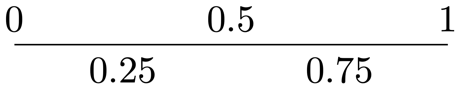
図 3.16 – 直線上のノード

\documentclass[tikz,border=10pt]{standalone}
\begin{document}
\begin{tikzpicture}
  \draw (0,0) --
    node [above, pos=0] {0}
    node [above, pos=0.5] {0.5}
    node [above, pos=1] {1}
    node [below, pos=0.25] {0.25}
    node [below, pos=0.75] {0.75}
  (4,0);
\end{tikzpicture}
\end{document}

---

図 3.17 – 非常にずれた配置

\documentclass[tikz,border=10pt]{standalone}
\usetikzlibrary{positioning}
\begin{document}
\begin{tikzpicture}[every node/.style = {inner sep=0pt}]
  \node (E) {E};
  \node (p) [right = 0pt of E] {p};
  \node (i) [right = 0pt of p] {i};
  \node (c) [right = 0pt of i] {c};
  \node (.) [right = 0pt of c] {.};
\end{tikzpicture}
\end{document}

---

図 3.18 – ベースラインに合わせた配置

\documentclass[tikz,border=10pt]{standalone}
\usetikzlibrary{positioning}
\begin{document}
\begin{tikzpicture}[every node/.style = {inner sep=0pt}]
  \node (E) {E};
  \node (p) [base right = 0pt of E] {p};
  \node (i) [base right = 0pt of p] {i};
  \node (c) [base right = 0pt of i] {c};
  \node (.) [base right = 0pt of c] {.};
\end{tikzpicture}
\end{document}

---

図 3.19 – デフォルトのピクチャ配置

\documentclass{article}
\usepackage{tikz}
\begin{document}
  \begin{tikzpicture}
    \node[circle, draw, inner sep=2pt] (label) {1};
  \end{tikzpicture}
  This is the first topic.
\end{document}

---

図 3.20 – TikZピクチャのベースライン配置

\documentclass{article}
\usepackage{tikz}
\begin{document}
  \begin{tikzpicture}[baseline=(label.base)]
    \node[circle, draw, inner sep=2pt] (label) {1};
  \end{tikzpicture}
  This is the first topic.
\end{document}

マクロを使用して同じ出力:

\documentclass{article}
\usepackage{tikz}
\DeclareRobustCommand{\circled}[1]{\tikz[baseline=(label.base)]{
  \node[circle, draw, inner sep=2pt] (label) {#1};}}
\begin{document}
  \circled{1} This is the first topic.
\end{document}

---

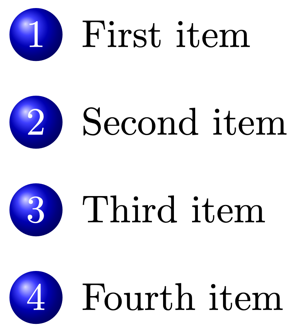
図 3.21 – 番号付きリストにおける装飾的なTikZ数字

\documentclass{article}
\usepackage{tikz}
\DeclareRobustCommand{\circled}[1]{%
  \tikz[baseline=(label.base)]{\node[circle,
    white, shading=ball, inner sep=2pt] (label) {#1};}}
\usepackage{enumitem}
\begin{document}
\begin{enumerate}[label=\circled{\arabic*}]
\item First item
\item Second item
\item Third item
\item Fourth item
\end{enumerate}
\end{document}

---

図 3.22 – ラベル付きのノード

\documentclass[tikz,border=10pt]{standalone}
\begin{document}
\begin{tikzpicture}[every label/.style = {scale=0.5}]
  \node[
    label = above:Graphics,
    label = left:Design,
    label = below:Typography,
    label = right:Coding,
    circle, shading=ball, ball color=blue!60,
      text=white] {TikZ};
\end{tikzpicture}
\end{document}

---

図 3.23 – ピン留めされたラベル付きのノード

\documentclass[tikz,border=10pt]{standalone}
\begin{document}
\begin{tikzpicture}[every pin/.style = {scale=0.5}]
  \node[
    pin = above:Graphics,
    pin = left:Design,
    pin = below:Typography,
    pin = right:Coding,
    circle, shading=ball, ball color=blue!60,
      text=white] {TikZ};
\end{tikzpicture}
\end{document}

---

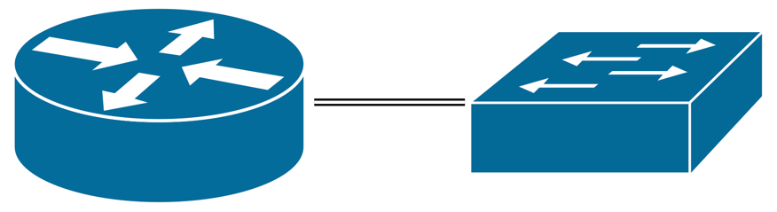
図 3.24 – ノード内の画像

\documentclass[tikz,border=10pt]{standalone}
\usetikzlibrary{positioning}
\begin{document}
\begin{tikzpicture}
  \node (router) [inner sep=0pt]
    {\includegraphics[width=2cm]{router.pdf}};
  \node (switch) [inner sep=0pt, right = of router]
    {\includegraphics[width=2cm]{switch.pdf}};
  \draw[double] (router) -- (switch);
\end{tikzpicture}
\end{document}

---

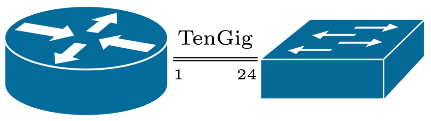
図 3.25 – 接続とラベル付きのノード内の画像

\documentclass[tikz,border=10pt]{standalone}
\usetikzlibrary{positioning}
\begin{document}
\begin{tikzpicture}
  \node (router) [inner sep=0pt]
    {\includegraphics[width=2cm]{router.pdf}};
  \node (switch) [inner sep=0pt, right = of router]
    {\includegraphics[width=2cm]{switch.pdf}};
  \draw[double] (router) --
    node [above, font=\scriptsize] {TenGig}
    node [font=\tiny, inner xsep=0pt,
      below right, at start] {1}
    node [font=\tiny,inner xsep=0pt,
      below left, at end] {24}
  (switch);
\end{tikzpicture}
\end{document}

次の章 へ進む.